


Z-Image Teleportation: Why Exact Replay Now Starts at Step 7
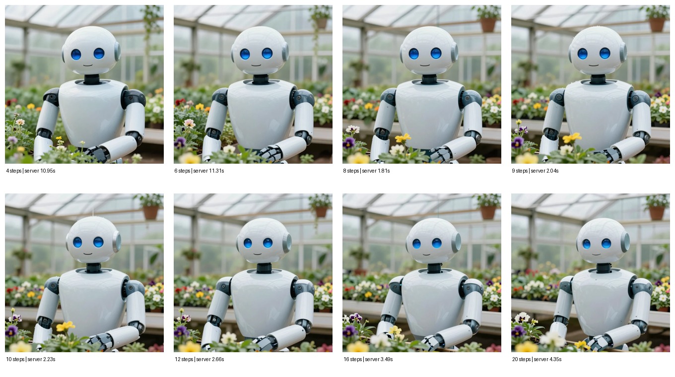
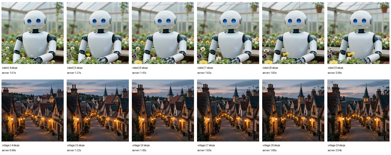
After moving Z-Image's normal default to 8 steps, the next question was teleportation. The site has a latent teleport path that can cache an intermediate latent and resume generation later. The parameter that matters most is where we resume.
There are two different ideas under the same "teleportation" label:
- **Exact-prompt replay**: cache a latent for the same prompt, seed, size, and step count, then resume that same denoising trajectory.
- **Compositional unit teleport**: combine cached latents for prompt pieces, then refine the combined latent into a new image.
The sweep showed a clean result: exact-prompt replay is production-useful, compositional unit teleport is still research.
Exact-prompt replay
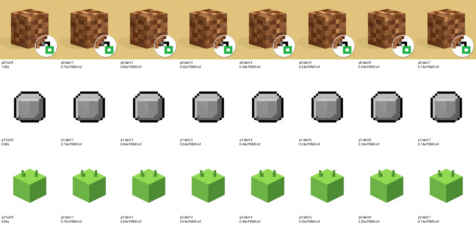
For the production path, we tested a full 8-step Z-Image generation and then replayed from cached latents captured after each earlier step. The prompt, seed, size, guidance, and step count stayed fixed.
| Resume step | Cached after step | Mean replay time at 512px | Quality vs full 8-step output | Verdict |
|---|---|---|---|---|
| 1 | 0 | 0.745s | Pixel-identical | Correct, but too much replay |
| 2 | 1 | 0.644s | Pixel-identical | Previous conservative default |
| 3 | 2 | 0.544s | Pixel-identical | Correct |
| 4 | 3 | 0.443s | Pixel-identical | Correct |
| 5 | 4 | 0.344s | Pixel-identical | Correct |
| 6 | 5 | 0.244s | Pixel-identical | Correct |
| 7 | 6 | 0.142s | Pixel-identical | New default |
Every exact replay setting produced the same pixels as the full 8-step generation. That is expected: we are not guessing a new latent; we are continuing the same trajectory from a cached point. Once the cache hit exists, starting at step 7 only reruns the final denoising step and VAE decode. On production, the first replay after a process restart can still pay a one-time compile warm-up; warmed replay measured 152 ms in the live API check.
So the production setting changed from:
LATENT_TELEPORT_START_STEP=2to:
LATENT_TELEPORT_START_STEP=7With the current 8-step Z-Image default, that means the server stores the latent after step 6 and resumes at step 7 on cache hits.
Compositional teleport
We also tested the more ambitious version: tokenize a new prompt into visual units, load cached unit latents, combine them with the tree combiner, then refine for 4, 6, 8, 10, 12, or 14 steps on a 20-step schedule.
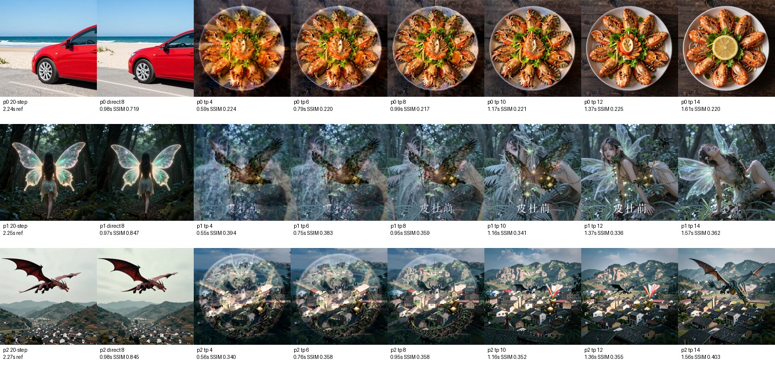
| Mode | Mean time at 512px | Mean SSIM vs 20-step reference | What happened |
|---|---|---|---|
| Direct 8-step generation | 0.974s | 0.803 | Strong baseline |
| Teleport, 4 refine steps | 0.563s | 0.319 | Fast, but visually wrong |
| Teleport, 6 refine steps | 0.768s | 0.320 | Still not enough structure |
| Teleport, 8 refine steps | 0.964s | 0.311 | As slow as direct 8 and worse |
| Teleport, 10 refine steps | 1.163s | 0.305 | More time, no useful gain |
| Teleport, 12 refine steps | 1.366s | 0.306 | Still weak |
| Teleport, 14 refine steps | 1.577s | 0.328 | Best compositional result, still not production-ready |
The image sheet makes the problem obvious. Unit-level teleport can preserve pieces of cached concepts, but it does not yet compose them into the requested scene reliably. On the car prompt, it teleports into a plate-of-food latent. On the fairy and dragon prompts, it often creates overlays and mixed compositions instead of a clean target image.
Code changes from the sweep
The sweep found two implementation issues in the research path:
- Z-Image `encode_prompt` returns prompt embeddings as a list, so cache population needed to normalize list outputs before storing embeddings.
- `CombinerConfig.refinement_steps` existed in the ablation grid but was not actually controlling the refinement count; fixed refinement now lines up the cached latent step with the denoising resume step.
Those fixes make the compositional benchmark honest, but they do not make compositional teleport a production default yet.
Decision
For production exact-prompt teleportation:
- Use `LATENT_TELEPORT_START_STEP=7`.
- Keep 8 total Z-Image steps as the normal generation default.
- Treat teleport cache hits as exact replay acceleration, not creative regeneration.
For compositional unit teleportation:
- Keep it experimental.
- Do not route normal user generations through it.
- Use direct 8-step Z-Image for quality per second until the latent combiner learns prompt-level composition instead of just blending cached unit trajectories.
The practical win is simple: exact-prompt replay can make repeated prompt/seed requests much faster without changing the image. The broader teleportation idea still needs model work before it beats direct generation.
Try CuteDSL
All CuteDSL services are powered by the $CUTEDSL token on Solana. Connect your wallet, deposit $CUTEDSL, and start making API calls in under a minute.
Need $CUTEDSL tokens? Buy $CUTEDSL on bags.fm — the fastest way to get tokens and start using accelerated AI inference.